Predict and verify Yes-Shares

The stability of municipal voting behavior presents a significant advantage from a result verification standpoint. Municipal ideological alignment generally shifts only gradually, allowing for the identification of historical referenda that exhibit approval patterns similar to those of current proposals. Leveraging this stability, we can make precise predictions and run simulations on voting sundays to estimate the expected outcomes based on historical data trends.

# Attach packages
library(plausi)
library(ggplot2)
library(dplyr)
library(tidyr)

# Municipality-codes ("BFS-Nummern") of selected municipalities
bfs_nrs <- c(6, 7, 10, 11, 12, 87, 219, 294, 181, 38, 60, 92, 119, 182, 218, 261)

Data Retrieval

Option 1: Retrieve voting results dynamically via swissdd from opendata.swiss

We can access all voting information on the federal level using the swissdd package.

# Install and attach package
devtools::install_github("politanch/swissdd")
library(swissdd)

# Retrieve results from the canton of Zurich for all federal votes from 2017-03-01 until 2020-09-27
results_raw <- swissdd::get_nationalvotes(from_date = "2017-03-01", to_date = "2020-09-27") |> 
  filter(canton_id == 1)

Option 2: Use the preloaded result_data included in the package

# Get historical package data
results_raw <- result_data

Data Wrangling

Some municipalities are more challenging to predict, because their voting patterns deviates significantly (e.g. the city of Zurich in our case). We address this by increasing their sample weight through upsampling.

# Introduce an artificial error
results <- results_raw |> 
  mutate(jaStimmenInProzent = ifelse(mun_id == 7 & id == 6310, jaStimmenInProzent + 15, jaStimmenInProzent))

# Transpose historical data into wide format (= one column per ballot / vote topic)
testdata <- results |> 
  filter(mun_id %in% bfs_nrs) |>  
  mutate(id = paste0("v", id)) |> 
  select(
    jaStimmenInProzent, 
    id, 
    mun_id, 
    mun_name
  ) |> 
  pivot_wider(
    names_from = id, 
    values_from = jaStimmenInProzent
  ) |>  
  drop_na()

# Upsampling
traindata <- testdata |> 
  mutate(ntimes = ifelse(mun_id %in% c(261, 12), 3, 1)) 

traindata <- as_tibble(lapply(traindata, rep, traindata$ntimes)) |> 
  select(-ntimes)

Prediction

We use the svmRadial model (SVM algorithm with a radial kernel) to predict the yes-shares, as it demonstrated the best performance in our benchmarks while maintaining a quick computation time.

# Set seed for reproducibility
set.seed(42)

# Predict results
predicted_results <- predict_votes(
  x = c("v6350", "v6310"),
  traindata = traindata, 
  testdata = testdata,
  method = "svmRadial", 
  geovars = c("mun_id", "mun_name")
)

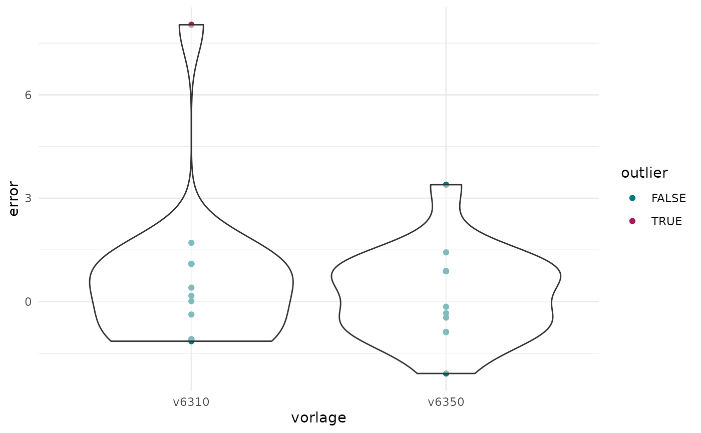
Detect Outliers

# Calculate the deviation of the reported result from the prediction and flag values that deviate by more than three RMSE as anomalous
gem_pred <- predicted_results |> 
  mutate(error = real - pred) |>  
  group_by(vorlage) |> 
  mutate(rmse = rmse(pred, real)) |>  
  mutate(error_rmse = error / rmse) |>    
  mutate(outlier = error_rmse > 3)

# Knonau with the anomalous result gets flagged
gem_pred %>% filter(outlier == TRUE)
#> # A tibble: 1 × 9
#> # Groups:   vorlage [1]
#>   mun_id mun_name  pred  real vorlage error  rmse error_rmse outlier
#>   <chr>  <chr>    <dbl> <dbl> <chr>   <dbl> <dbl>      <dbl> <lgl>  
#> 1 7      Knonau    46.2  54.2 v6310    8.04  2.23       3.60 TRUE

# Plot the deviations
ggplot(gem_pred, aes(vorlage,error)) +
  geom_point(aes(color = outlier)) +
  geom_violin(alpha = 0.5) +
  scale_colour_manual(values = c(
    "TRUE" = "#B01657",
    "FALSE" = "#00797B"
  )) +
  theme_minimal()